Training data and network

The CNN never sees a measured curve during training. Every batch is simulated on the fly, so there are no dataset files: reflectolearn train draws film and substrate parameters, computes R(q) with a batched Abeles transfer-matrix engine (Névot-Croce roughness, complex SLD), and distorts the curves the way an instrument would. The ranges below are the defaults in reflectolearn/config.py, which reflectolearn config writes out; every one can be changed in the config file.

What is drawn

Uniformly, per curve:

	range
film thickness	10–1200 Å
film roughness	0–15 Å
film SLD	5–100 ×10⁻⁶ Å⁻²
substrate SLD	18–22 ×10⁻⁶ Å⁻² (Si is about 20)
substrate roughness	1–6 Å

The curve covers 2θ = 0.05–15° at 1.54 Å on 2000 q points. The network predicts the three film parameters; the substrate is simulated but not predicted.

Domain randomization

A curve simulated from the film alone is cleaner than any measurement. To make the network robust to the difference, the generator and the augmentor add effects it is not asked to predict:

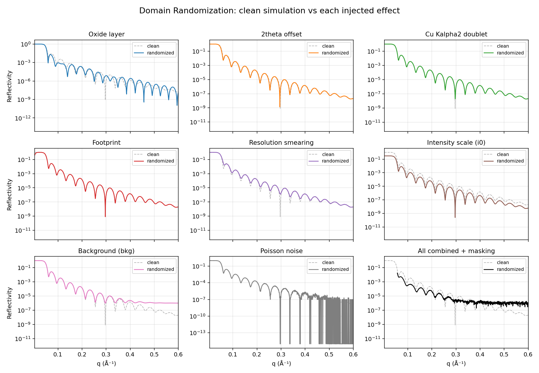
In the forward model, per curve (augmentation section of the config):

• a native-oxide layer on top of the film, present with probability 0.7, 0–40 Å thick, SLD 5–25;
• a 2θ zero offset of ±0.02°;
• the Cu Kα2 doublet, with a Kα2/Kα1 ratio drawn from 0–0.5.

Then instrument effects, each switched on for a batch with probability prob (0.9):

• footprint attenuation at low angle (beam width 0.005–0.015 mm, sample length 5–30 mm);
• Gaussian resolution smearing, σ_q = 0.0001–0.006 Å⁻¹;
• intensity scale 0.8–1.2 and a background of 10⁻⁸–10⁻⁵;
• Poisson counting noise at 10⁵–10⁸ counts at R = 1;
• up to 5% of the points cut at each end of the curve, recorded in a mask.

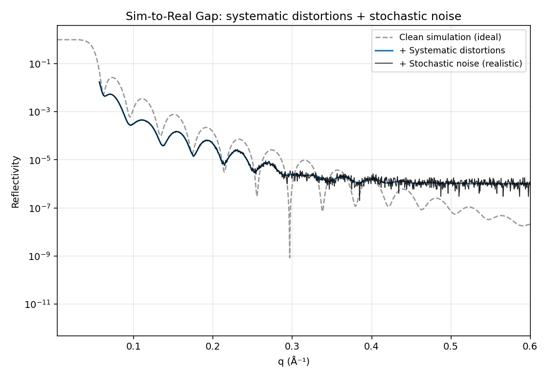
The curve is then normalized to its maximum and taken as log10; the masked points are set to a fixed floor so the network sees one consistent "no data" value.

The network

XRRPhysicsModel takes two channels, the log10 curve and its mask, adds random Fourier features of q, runs a stack of 1D convolution blocks (kernel 7, batch norm, LeakyReLU, dropout, max-pool by 2; channels double up to eight times the first), averages over q and maps the result to the three normalized film parameters with a small MLP. Training minimizes the MSE on those normalized values.

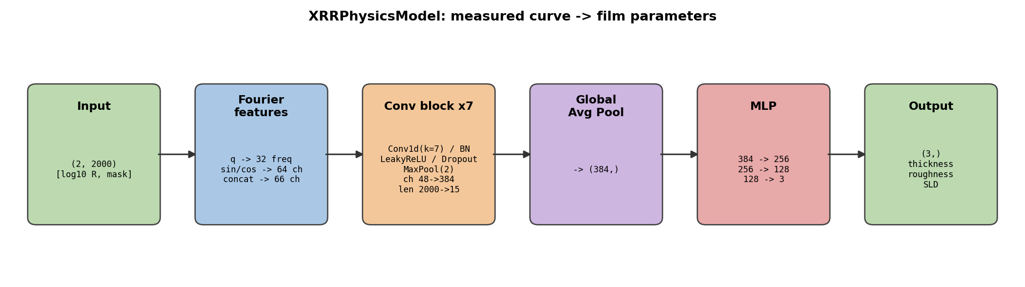
The diagram is drawn from the repository's config.yaml (48 channels, depth 7, MLP width 256, the dimensions of the trained model). The code defaults that reflectolearn config writes are 64 channels, depth 6 and MLP width 512; python -m reflectolearn.report.figures redraws the diagram for whatever config.yaml it finds in the current directory.

What this does not cover

The training curves are one film, an optional oxide and a substrate, from the same physics family as the fit. Interdiffusion, density gradients, multilayers, a non-Gaussian beam and detector nonlinearity are not simulated, so a measured curve with them is outside what the network has seen.